Working with Alerts in Power BI

Knowing about changes to important metrics quickly some time can help you taking quick decisions or help you keep eyes on things you care most.

With data driven alerts in Power BI, you can now get notifications when a metric you care about on your dashboard exceeds a set threshold.

Alert notifications will be sent to you as an email, and appear in your notification center on the web and in mobile apps.

You can set alerts for your numeric tiles featuring cards and gauges only. You have control over how often you want to be notified about your data, and whether you want to receive an email when your data goes beyond the limits you set.

Only you can see the alerts you set, even if you share your dashboard.

Alerts only work on data that is refreshed. When data refreshes, Power BI looks to see if an alert is set for that data. If the data has reached an alert threshold, an alert is triggered.

Alerts only work with numeric data types.

Alerts only work on data that is refreshed. They do not work on static data.

Today we will see how to work with Alert feature in Power BI.

Login to your Power BI using your credentials.

Switch to your Dashboard.

I have one ready to use dashboard from my previous post to show Alert feature I am using the same.

As discussed above it works only for Numeric & Gauges Tiles only, for others you will not get even the Alert option.

Luckily I have one on my Dashboard, if want to learn how to create Numeric Tiles or more details on working with Power BI you can refer to any of my previous posts on Power BI. However you can find here one direct Link to the topic in question.

You see I have selected my Numeric Tile in below screen shot.



How to Set Data Alerts:

From a dashboard tile, select the ellipses.

Select the bell icon  to add one or more alerts.



Click on Add Alert Rule.

To start, ensure the Active slider is set to ON, and give your alert a title.



 

Set your Condition, Threshold, and Notification Frequency also don’t forget to tick on send me mail too.

Click on Save to save your Alert.

 

Receiving alerts:

When the data being tracked reaches one of the thresholds you've set, several things will happen.

Power BI checks to see if time have lapsed or more than depending on the option you selected since the last alert was sent.

As long as the data is past the threshold, you'll get an alert every hour or every 24 hours depending on option you selected.

If you've set the alert to send you an email, you'll find something like as shown in below screen, this in your Inbox.

 



 

Power BI will add a message to your Notification center and adds a new alert icon to the applicable tile as shown in below screen.



 

Access to your Notification.



 

 

Manage alerts:

There are three ways to manage your alerts:

From the dashboard tile

From the Power BI Settings menu

On an individual tile in the Mobile App



 

As we have seen above how to create Alerts follow same steps to access Alert Window.

At the Left click on Expand make Necessary Modifications and save.

At the right select the trashcan to delete the Alert.

Select cancel to return to previous window.

 



From here you can turn alerts on and off, open the Manage alerts window to make changes, or delete the alert.

 

That’s all for today.

I will come up with more details in my upcoming posts.

Till then keep exploring and learning.

 

 

Now Power BI Added to Microsoft Trust Center

The Microsoft Trust Center provides a single point of reference for cloud trust resources, including documentation of our adherence to international and regional compliance certifications and attestations, privacy and data protection policies and processes, data transfer and location policies, and security features and functionality.

When you entrust your data to the Microsoft Cloud, you will have questions. Where is it? Who can access it? What is Microsoft doing to protect it? How can you verify that Microsoft is doing what it says?

For more information see this Link: https://www.microsoft.com/en-us/trustcenter

https://powerbi.microsoft.com/en-us/blog/power-bi-added-to-microsoft-trust-center/

The Power BI service is built on Azure, Microsoft’s cloud computing platform, and leverages Azure’s robust set of security technologies and practices. These help ensure that Power BI is resistant to attack, safeguards user access, and helps secure your data through encrypted communications.

As a Power BI customer, you know, through clearly stated policies and procedures, where your customer data is stored and how we help secure it, as well as who can access it and under what circumstances.

How to add Video Tile on Power BI Dashboard

Previously, a Video Tile released by BI supports YouTube videos. Video tiles allow you to customize your dashboard and add a bit of personal look.

Now the video tile supports Vimeo videos too.

Add a video tile by selecting Add widget from the top right of the dashboard.



Select Video from Add Tile window.



Press Next Button.



Provide your Title and Subtitle for the Video Tile.

Provide your YouTube or Vimeo video URL.

If required provide custom Link and other properties.

Select Apply to complete your action.

Vimeo URLs come in several different formats this supports most, but not all of these formats. In case your URL doesn’t works try for next format.

I have posted several posts related to Power BI, you can find them using below Links.

Microsoft Power BI – Part – I

Introduction to Power BI and Creating Report from Excel Data, Local Files.

Microsoft Power BI – Part – II

Introduction to few Features of Power BI

Microsoft Power BI – Part – III

Power BI Desktop, Creating Dataset & Reports from In Premise Database installation

Microsoft Power BI – Part – IV

Power BI Gateway usage

Microsoft Power BI – Part – V

Scheduling Refresh of Dataset & Report created using In Premise Database

Microsoft Power BI – Part – VI

Power BI Content Pack

Microsoft Power BI – Part – VII

Power BI Mobile App

Microsoft Power BI – Part – VIII

Power BI Content Pack

Microsoft Power BI – Part – IX

Power BI Publisher for Excel

Microsoft Power BI – Part – X

Analyse in Excel (preview)

 

 

Power BI - Overview and Learning

Microsoft Power BI is a collection of online services and features that enables you to find and visualize data, share discoveries, and collaborate in intuitive new ways. There are two experiences now available for Power BI: the new experience, generally referred to as Power BI, and the previous experience which is referred to as Power BI for Office 365.

 

Please check this link:- Overview and Learning



 

 

Microsoft Power BI – Part IX

Continuing from my previous post. Today we will see usage of Power BI Publisher for Excel.

In case you have missed my previous posts here I present the link to all previous posts below.

Microsoft Power BI – Part – I

Introduction to Power BI and Creating Report from Excel Data, Local Files.

Microsoft Power BI – Part – II

Introduction to few Features of Power BI

Microsoft Power BI – Part – III

Power BI Desktop, Creating Dataset & Reports from In Premise Database installation

Microsoft Power BI – Part – IV

Power BI Gateway usage

Microsoft Power BI – Part – V

Scheduling Refresh of Dataset & Report created using In Premise Database

Microsoft Power BI – Part – VI

Power BI Content Pack

Microsoft Power BI – Part – VII

Power BI Mobile App

Microsoft Power BI – Part – VIII

Power BI Content Pack

Sharing key Excel insights just got easier. Save snapshots of important PivotTables, Charts, cell ranges, and more from across all of your spreadsheets to a single location quickly with the Power BI publisher for Excel. Simply highlight the elements you want to save, then click the "Pin to" button: now you’ve got a powerful web dashboard that you can share with everyone in your organization.

Let us see how we can use this feature.

Login to Power BI with your credentials.



From Download Menu Section choose Power BI Publisher for Excel.

Or visit Link: https://powerbi.microsoft.com/en-us/excel-dashboard-publisher/



Select your desired Excel Version 32 or 64 bit as installed on your PC and download the Package.

Close your Excel and Install the Package and follow on screen guide.

After Installation when you open your Excel First time after Installing the Package. You will get similar to below screen.



Sign in with your Power BI Credentials.



 



 



I have created a Pivot in excel as below which I want to share on my Desktop.



Select the Region/Range that you wish to publish from Power BI choose Pin, as shown below.



In my case I have already pined so confirmation Dialog Box is taken else it will Pin the Selected Range as a snapshot on selected Workspace.



Make sure you select right Workspace before you Pin.



After Publishing you will get confirmation as below.



Using the Link, Login with your credentials to the Power BI and switch to the Dashboard on which you published.



This way you can Pin Snapshot of PivotTables, Charts, cell ranges, and more. You can update existing with new one and manage all your Pins.



Save your Excel and Exit.



Try useful feature.

I will come up with more details in my future posts.

Till then keep practicing and learning using online Blogs, help and documents.

Create a Power View report

In the previous post, we created an Excel workbook with a PivotTable containing data about Olympic medals and events. If you didn’t saw the previous post you can access from here.

Use hierarchies in PivotTables

In this post, we will create a Power View report to visually represent the Olympics data.

In Excel, click INSERT > Reports > Power View Reports.





Select City from Host & Sport from Medal Table. Apply Count (Not Blank) to Sport Field using dropdown list next to Field Name.

From design switch the Visualization to Map.

On the map, blue circles of varying size indicate the number of different sport events held at each Olympic Host location.

Drag Season Field to Color area. This will add different colors for different Seasons. In our case summer/Winter Red/Blue colors.

Just in few clicks now we have a Power View report that visualizes the number of sporting events in various locations, using a map, color-coded based on season.

Will come with more details in my upcoming posts, till then stay tuned, keep learning and practicing.

Power View in Excel 2013

Power View is an interactive data exploration, visualization, and presentation experience that encourages intuitive ad-hoc reporting.

Power View is a feature of Microsoft Excel 2013, and of Microsoft SharePoint Server 2010 and 2013 as part of the SQL Server 2012 Service Pack 1 Reporting Services Add-in for Microsoft SharePoint Server Enterprise Edition.

Power View has these features, as part of Power BI for Office 365:

• Create Power View sheets in Excel and then view them in the Power BI Windows Store app.


• View Power View in Excel sheets in your browser, without installing Silverlight.

Data sources for Power View

In Excel 2013, you can use data right in Excel as the basis for Power View in Excel and SharePoint.

When you add tables and create relationships between them, Excel is creating a Data Model behind the scenes.

A data model is a collection of tables and their relationships reflecting the real-world relationships between business functions and processes—for example, how Products relates to Inventory and Sales.

You can continue modifying and enhancing that same data model in Power Pivot in Excel, to make a more sophisticated data model for Power View reports.

With Power View you can interact with data:

• In the same Excel workbook as the Power View sheet.


• In data models in Excel workbooks published in a Power Pivot Gallery.


• In tabular models deployed to SQL Server 2012 Analysis Services (SSAS) instances.


• In multidimensional models on an SSAS server (if you’re using Power View in SharePoint Server).

Recall from my previous post Creating My First Report using PowerPivot, I will be using same Data Model to demonstrate the feature of Power View, also same report in different format.

Let’s design Customer wise Sales Report using Power View.


I am using the same Workbook which we used for PowerPivot creating Matrix report for Item Vs Customer Sales.

From Insert Tab choose Power View Reports in ribbon.

Remember this workbook already having Data Model with tables Customer, Item, Cust. Ledger Entry & Item Ledger Entry. One which we created during our previous exercise during walkthrough of PowerPivot.

We already have Relationship defined between Customer & Item Ledger Entry (No. -> Source No.), also Item & Item Ledger Entry (No. -> Item No.).


You can View the Relationship using Relationship from Ribbon Power View Tab.

Once the Power View Sheet is inserted the Power View Tab will be Visible.

This will list the two relations which we created earlier in previous exercise post.

However we will be requiring one more relationship for this report. Add using New button on Manage Relationship window.

Enter the Relation for Customer & Cust. Ledger Entry (No. -> Customer No.).

You can see all the 4 tables are listed in Field List Pane.

Arrange the Fields from respective tables as shown in above screenshot.

Arrange the fields as shown in above screenshot.

Design of your report should be similar to one shown in below screenshot.


Resize the Table area to fit the area and the way you want to represent the data.

When a Customer is selected in Title Area, below two tables show the Item Sales Quantity & Total Value for the selected Customer.

You can add fields in the Filter Pane to slice the data accordingly.

I will come up with more details in my upcoming posts.

Till then stay tuned and keep practicing.

Troubleshooting: Power Pivot Ribbon Disappears

In rare cases, the Power Pivot ribbon will disappear from the menu if Excel determines that the add-in is destabilizing to Excel. This might occur if Excel closes unexpectedly while the Power Pivot window is open. To restore the Power Pivot menu, do the following:

• Go to File > Options > Add-Ins.

In the Manage box, click Disabled Items > Go

• Select Microsoft Office Power Pivot in Microsoft Excel 2013 and then click Enable.

If the previous steps do not restore the Power Pivot ribbon, or if the ribbon disappears when you close and reopen Excel, try the following:

• Close Excel.


• Point to Start > Run and then type regedit.


• In Registry Editor, expand HKEY_CURRENT_USER > Software > Microsoft > Office > 15.0 > User Settings.


• Right-click PowerPivotExcelAddin and then click Delete.


• Scroll back up to the top of Registry Editor.


• Expand HKEY_CURRENT_USER > Software > Microsoft > Office > Excel > Addins.


• Right-click PowerPivotExcelClientAddIn.NativeEntry.1 and then click Delete.


• Close Registry Editor.


• Open Excel.


• Enable the add-in using the steps at the top of this article.

Start the Power Pivot in Microsoft Excel add-in

Power Pivot in Microsoft Excel 2013 is an add-in you can use to perform powerful data analysis in Excel. The add-in is built into Excel, but by default, it's not enabled. Here’s how you enable Power Pivot before using it for the first time.

• Go to File > Options > Add-Ins.

In the Manage box, click COM Add-ins> Go

• Check the Microsoft Office Power Pivot in Microsoft Excel 2013 box, and then click OK. If you have other versions of the Power Pivot add-in installed, those versions are also listed in the COM Add-ins list. Be sure to select the Power Pivot add-in for Excel.

The ribbon now has a Power Pivot tab

PowerPivot Creating a Data Model in Excel 2013

Before you can create a PivotTable, you'll need some data. Let's get some data from the Navision database.

In Excel, open a blank workbook.





You have several options for getting data from no of sources.

Recall from my earlier post where we accessed data using web service in Excel.

Viewing Page Data in Excel Using PowerPivot (OData)

Let us see what other options are available to us.


In today’s Example I will be connecting with SQL but will access Navision 2015 Database.

Follow the Steps below:


Give meaningful name to your connection in my case I have used Nav2015DB_SQL_Connection.

Select the SQL Server to which you wish to connect in my case I have used INDEL-AXT5283N1, basically this is the SQL Server installed on my Laptop.


Specify the Login method, I am using Windows Authentication, if required you can use SQL Server Authentication. In later case you will have to specify your User Name & Password.

Select the Database to Connect, I have selected Demo Database NAV (8-0) Std. Database for Navision 2015.

Click the Test Connection button, If everything is ok you will get Connection Succeed Message, as shown in above screen shot.

Press Next for next step.


In this screen you have option to either import data from Tables and Views or you can Write Query to fetch data for import.

In my case for this example I am importing data from tables.

Select option – Select from a list of tables and views to choose the data to import and Press Next for next step.


I have Selected two Tables Cust. Ledger Entry & Customer.

Select Related Tables button ensure to select if any other tables related to this Table.

In my case not applicable. Click Finish to add data to the Data Model/ Import the data of these two tables.

Select Close to return to Data Sheet imported after this operation.

Here you see your Data for these two tables have been imported in two sheets.

What happened?

You might not have realized it yet, but you’ve just created a data model. It's created automatically when you import or work with multiple tables simultaneously in the same PivotTable report. The model is mostly transparent in Excel, but you can view and modify it directly using the Power Pivot add-in. In Excel, the presence of a data model is evident when you see a collection of tables in the PivotTable Fields list. There are several ways to create a model.

I will come up with more details in my next post.

PowerPivot for Excel

Power Pivot: Powerful data analysis and data modelling in Excel

Power Pivot is an Excel add-in you can use to perform powerful data analysis and create sophisticated data models. With Power Pivot, you can mash up large volumes of data from various sources, perform information analysis rapidly, and share insights easily.

In both Excel and in Power Pivot, you can create a Data Model, a collection of tables with relationships. The data model you see in a workbook in Excel is the same data model you see in the Power Pivot window. Any data you import into Excel is available in Power Pivot, and vice versa.

How the data is stored

The data that you work on in Excel and in the Power Pivot window is stored in an analytical database inside the Excel workbook, and a powerful local engine loads, queries, and updates the data in that database. Because the data is in Excel, it is immediately available to PivotTables, Pivot Charts, Power View, and other features in Excel that you use to aggregate and interact with data. All data presentation and interactivity are provided by Excel; and the data and Excel presentation objects are contained within the same workbook file.

Power Pivot supports files up to 2GB in size and enables you to work with up to 4GB of data in memory.

Download PowerPivot for Excel

• Go to the Microsoft Web site (http://go.microsoft.com/fwlink/?LinkId=258219).


• Download either the x86 (32-bit) or the x64 (64-bit) version of PowerPivot_for_Excel.msi installation program. The version of the add-in must correspond to the version of Excel on your computer.

To determine whether you are using 32-bit or 64-bit software, look at the C:\Program Files folder.

Download x86\PowerPivot_for_Excel_x86.msi if you have only “C:\Program Files”. Both the operating system and Office 2010 are 32-bit.

Download x86\PowerPivot_for_Excel_x86.msi if you have both “C:\Program Files” and “C:\Program Files (x86)”, and the Excel.exe application file is found in “C:\Program Files (x86)\Microsoft Office\Office14”. The operating system is 64-bit, but the version of Office is 32-bit.

Download x64\PowerPivot_for_Excel_amd64.msi if you have both “C:\Program Files” and “C:\Program Files (x86)”, and the Excel.exe application file is found in “C:\Program Files\Microsoft Office\Office14”. Both the operating system and Office 2010 are 64-bit.

Install PowerPivot for Excel

• Double-click the .msi file to start the Setup wizard. Click Run.


• Click Next to get started.


• Accept the license agreement, and then click Next.


• Enter your name, and then click Next.


• Click Install.

Click Finish.

Verify Installation

Start Excel. After you install the add-in, you can open the PowerPivot window by clicking the PowerPivot tab on the Excel ribbon, and then clicking PowerPivot Window.

An empty PowerPivot window opens over the Excel application window.

You can then use the Import Wizard to add tables of data, create relationships between the tables, enrich the data with calculations and expressions, and then use this data to create PivotTables and PivotCharts.

Stay tuned for more information in my upcoming posts.

Viewing Page Data in Excel Using PowerPivot (OData)

Here I will discuss how you can use OData to expose a Microsoft Dynamics NAV 2015 page as a web service and then analyse the page data using Microsoft PowerPivot for Excel 2013.

With OData and PowerPivot, you gain access to a powerful set of tools and technologies for data exchange and analysis.

This walkthrough illustrates the following tasks:

• Publishing a Microsoft Dynamics NAV page as a web service.


• Verifying web service availability from a browser.


• Using the PowerPivot add-in for Excel to import the table data as a new worksheet.


• This procedure also includes optional instructions about how to use a web service access key.


• Creating a PivotTable from the worksheet, selecting relevant fields, and then organizing and formatting the data to highlight strategic data.

Optional:

If you want to use a web service access key to authenticate access to the web service, Microsoft Dynamics NAV must meet the following requirements:

The Microsoft Dynamics NAV Server is configured to authenticate users by using the NavUserPassword credential type.

There is a Microsoft Dynamics NAV user account that has a web service access key.

You can find more details in my earlier post here

Publishing a Page as a Web Service

You can publish a web service by using the Microsoft Dynamics NAV Web client or the Microsoft Dynamics NAV Windows client.

To register and publish a page as a web service

• Open the RoleTailored client and connect to the CRONUS International Ltd. company.


• In the Search box, enter Web Services, and then choose the related link.


• In the Web Services page, choose New.


• In the Object Type column, select Page. In the Object ID column, enter 21, and in the Service Name column, enter Customer.

This exposes the Customer Card page as an OData web service.

• Select the check box in the Published column.

Choose the OK button to close the New - Web Services page.


Verifying the Web Service’s Availability

Security Note

After publishing a web service, verify that the port that web service applications will use to connect to your web service is open. The default port for OData web services is 7048. You can configure this value by using the Microsoft Dynamics NAV Server Administration Tool.

To verify availability of a Microsoft Dynamics NAV web service

Start Windows Internet Explorer.

In the Address field, enter a URI using the following format: http://Server : WebServicePort/ServerInstance/OData/

Server is the name of the computer that is running Microsoft Dynamics NAV Server.

WebServicePort is the port that OData is running on. The default port is 7048.

ServiceInstance is the name of the Microsoft Dynamics NAV Server instance for your solution. The default name is DynamicsNAV80.

For example, if the Microsoft Dynamics NAV Server is running on the computer that you are working on, you can use: http://localhost:7048/DynamicsNAV80/OData/

In my case: - http://indel-axt5283n1.tecturacorp.net:8048/DynamicsNAV80/OData/

The browser should now show the web service that you have published, as shown in the following illustration.


Note

If the browser cannot find the web service, it may indicate that the specified Microsoft Dynamics NAV Server instance is not running.

Make Sure Enable OData Services is checked.

Importing Microsoft Dynamics NAV Data into Excel

In the following procedures, you use PowerPivot to import Microsoft Dynamics NAV data into Excel. If you will be using a web service access key for authentication, only perform the second procedure; otherwise, only perform the first procedure.

To import Microsoft Dynamics NAV data into Excel

Start Microsoft Excel.

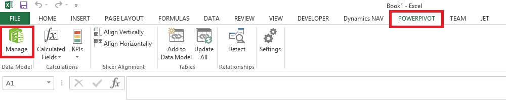
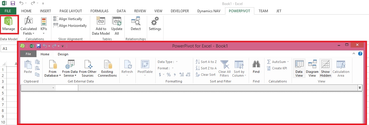
In Excel, on the PowerPivot tab, choose Manage.


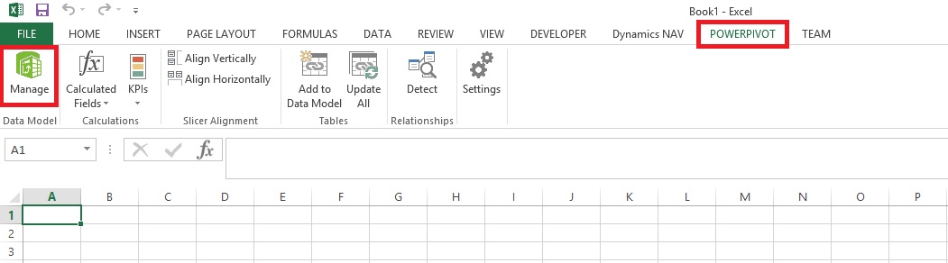
This opens the PowerPivot for Excel window.

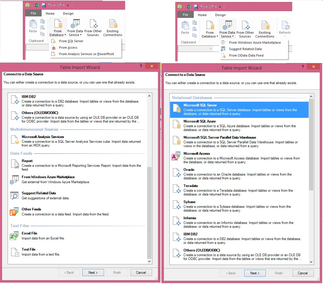
In PowerPivot, on the Home tab, choose Get External Data, choose From Data Service, and then choose From OData Data Feed.

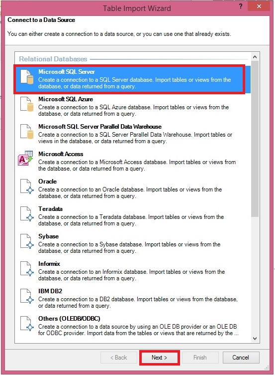
The Table Import Wizard opens.


If your Microsoft Dynamics NAV implementation requires that you use a web service access key, you must specify the NavUserPassword credentials as described in the following steps:

In the Advanced dialog box, in the Security section, set the Integrated Security field to Basic. If your OData is configured to use SSL, then set the field to SSPL.

In the Password field, type the web service access key.

In the UserID field, type the user name for the Microsoft Dynamics NAV user account. For this walkthrough, use NavTest.

In the Source section, in the Service Document URL field, type the URL for the OData web service that you verified in the previous procedure, for example, http://localhost:7048/DynamicsNAV80/OData/.

In my case: - http://indel-axt5283n1.tecturacorp.net:8048/DynamicsNAV80/OData/

Choose the OK button to return to the Table Import Wizard.

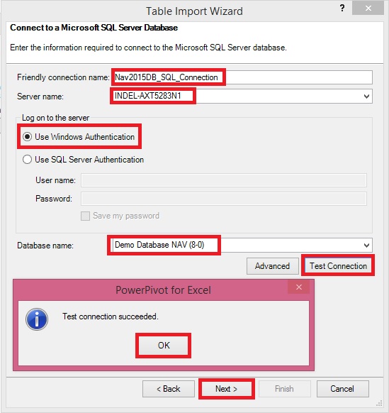
In the Connect to a Data Feed page, in the Data Feed Url field, enter the OData URI that you verified in the previous procedure.


Choose the Next button.

Important: The URI must end with a slash (/) as shown in the example.

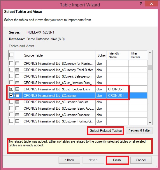
Verify that Customer appears in the Source Table column.

Select the check box next to the Customer web service, and then choose Finish.

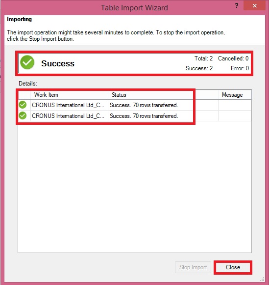
After you see the Success message, choose the Close button.


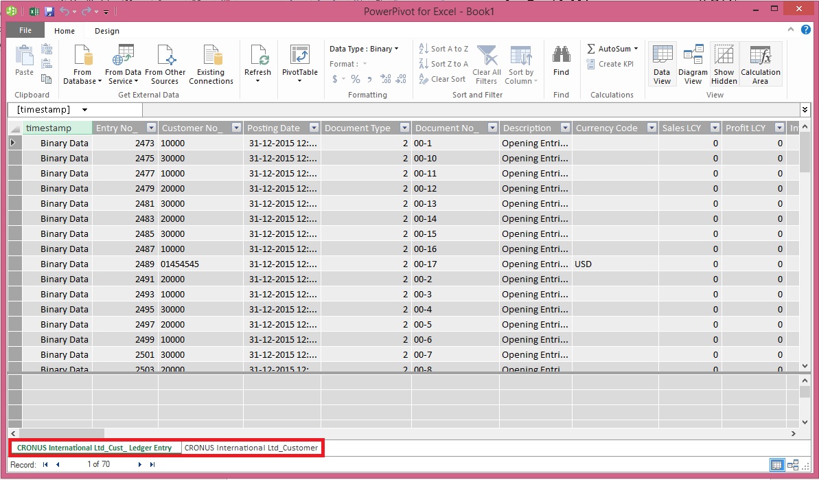
The data from the Customer OData web service displays, and you can use the data to build pivot-based views in the Excel workbook.

Creating a PivotTable Containing Key Microsoft Dynamics NAV Data

In this procedure, you use the Excel workbook with data from the Customer web service to create a PivotTable from the worksheet. You select relevant fields and then organize and format the data to highlight strategic data. Building a pivot table is a way to select and arrange data so as to highlight and focus on key elements.

To create a PivotTable

In Excel, select the cell where you want the PivotTable located.

In the ribbon, choose the Insert tab, and then in the Tables group, choose PivotTable.

In the Create PivotTable dialog box, select Use an external data source, and then choose the Choose Connection button.

In the Existing Connections dialog box, on the Connections tab, under Connections in this Workbook, choose the data feed for your OData web service, and then choose the Open button.


Choose the OK button to add the PivotTable to the Excel worksheet.

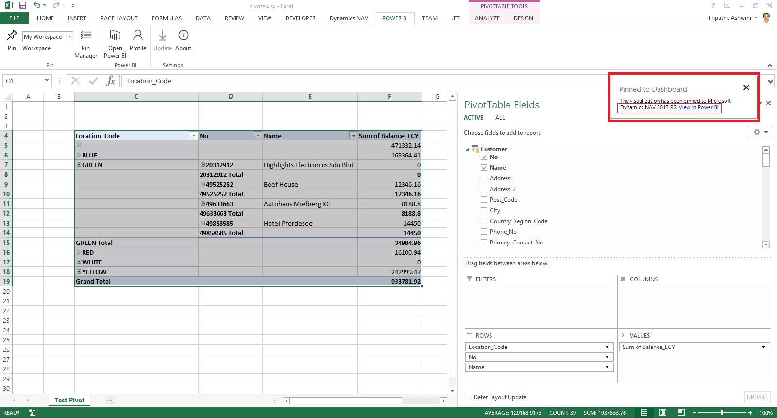
The PowerPivot Field pane on the right side includes a list of fields from the Customer web service that where imported from PowerPivot.

In the PowerPivot Field List pane, choose Location_Code.

Tip

To quickly find a field in the field list, type part or all of the field name in the Search text box that is above the list of fields, and then press Enter to highlight the first field that contains the text. You can then choose the right arrow to proceed to the next field, and so on.

Select the Balance_LCY field.

Select the Name field.

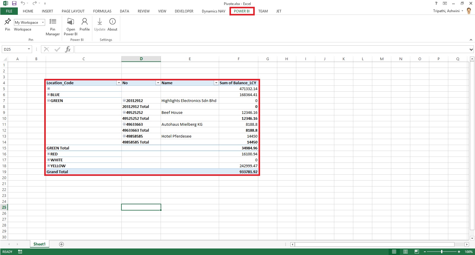
You can now see the data in the body of the worksheet, as shown in the following illustration.

The PivotTable shows customers by location and individual customer balances, and also adds the balances by location. To make the information more readable, you can update the headings on the PivotTable.


Select the cell that has the heading Sum of Balance_LCY, and then, in the formula field, type Balance.

Select the cell that has the heading Row Labels, and then in the formula field, type Customers by location.

Select the empty cell that is below the Customers by location cell, and then, in the formula field, type Location not specified.

The above illustration shows how the worksheet looks after you make these changes.

Next Steps

Now that you have created your PivotTable, you can continue to enhance the data to make it more useful and readable. You can:

Add a column to the data that shows average balance by region.

Enhance data presentation with a graph.

Post the data in a Microsoft SharePoint environment with live data from Microsoft Dynamics NAV 2015.