Wednesday 30 September 2015

Basics of Power Pivot for Excel – 2013

Dear friends, I have published couple of posts on this topic. I will be adding more advanced features and details related to this in my upcoming posts.

For your ready reference below I present Links to those posts.

PowerPivot for Excel

Start the Power Pivot in Microsoft Excel add-in

Troubleshooting: Power Pivot Ribbon Disappears

PowerPivot Creating a Data Model in Excel 2013

Adding more tables to the Data Model using Existing Connection – In PowerPivot

Add relationships to Data Model in PowerPivot

How to add Filter for data retrieval in PowerPivot Data model.

Create a calculated column in PowerPivot

Creating My First Report using PowerPivot

In Excel 2013, PowerPivot and Power View are no longer separate add-ins that need to be downloaded and installed. These add-ins are natively included.

PowerPivot in Excel 2013 is functionally very similar to the PowerPivot add-in for Excel 2010.

PowerPivot is an add-in that lets end users gather, store, model, and analyze large amounts of data in Excel. Power View provides intuitive data visualization of PowerPivot models and SQL Server Analysis Services (SSAS) tabular mode databases.

If you're unfamiliar with either PowerPivot or Power View, I encourage you to first review my previous post links provided above to understand the basics.

Some parts of the PowerPivot architecture is embedded inside of Excel 2013.

  • The PowerPivot version in Excel 2013 no longer uses a separate PowerPivot Fields list. Instead, the built-in PivotTable Fields list is used. This means that some capabilities from the Excel 2010 add-in (e.g., searching for fields by name, creation of slicers from the field list, surfacing of column descriptions when hovering over a field) are no longer available.

  • Workbooks with PowerPivot models are no longer limited to 2GB in size in Excel 2013. However, the 2GB limit still applies to workbooks that will be published to SharePoint.

  • In Excel 2013, a refresh of a PivotTable or PivotChart will, by default, initiate a refresh of the underlying data connections in the Data Model. This is very different from Excel 2010, where a PivotTable refresh only re-queries the model. The new refresh behaviour can be changed by clicking Connections on the Data tab, selecting Properties, and clearing the Refresh this connection on Refresh All check box.

  • Stay tuned for more information on this topic. Till then keep practicing & exploring.

  • In Excel 2013, a Power View "report" is a worksheet rather than an .rdlx file. There's no concept of multiple report views. Instead, multiple Power View worksheets can be created within a single Excel workbook.


Stay tuned for more information on this topic. Till then keep practicing & exploring.

Troubleshooting: Power Pivot Ribbon Disappears

In rare cases, the Power Pivot ribbon will disappear from the menu if Excel determines that the add-in is destabilizing to Excel. This might occur if Excel closes unexpectedly while the Power Pivot window is open. To restore the Power Pivot menu, do the following:

  • Go to File > Options > Add-Ins.


In the Manage box, click Disabled Items > Go
PowerPivot-29

  • Select Microsoft Office Power Pivot in Microsoft Excel 2013 and then click Enable.


If the previous steps do not restore the Power Pivot ribbon, or if the ribbon disappears when you close and reopen Excel, try the following:

  • Close Excel.

  • Point to Start > Run and then type regedit.

  • In Registry Editor, expand HKEY_CURRENT_USER > Software > Microsoft > Office > 15.0 > User Settings.

  • Right-click PowerPivotExcelAddin and then click Delete.

  • Scroll back up to the top of Registry Editor.

  • Expand HKEY_CURRENT_USER > Software > Microsoft > Office > Excel > Addins.

  • Right-click PowerPivotExcelClientAddIn.NativeEntry.1 and then click Delete.

  • Close Registry Editor.

  • Open Excel.

  • Enable the add-in using the steps at the top of this article.

Start the Power Pivot in Microsoft Excel add-in

Power Pivot in Microsoft Excel 2013 is an add-in you can use to perform powerful data analysis in Excel. The add-in is built into Excel, but by default, it's not enabled. Here’s how you enable Power Pivot before using it for the first time.

  • Go to File > Options > Add-Ins.


In the Manage box, click COM Add-ins> Go
PowerPivot-26

  • Check the Microsoft Office Power Pivot in Microsoft Excel 2013 box, and then click OK. If you have other versions of the Power Pivot add-in installed, those versions are also listed in the COM Add-ins list. Be sure to select the Power Pivot add-in for Excel.


PowerPivot-27
The ribbon now has a Power Pivot tab
PowerPivot-28

Creating My First Report using PowerPivot

In my earlier posts we have created the Data model for Analysis.

If you missed them you can follow below links to refresh all information.

PowerPivot for Excel

PowerPivot Creating a Data Model in Excel 2013

Adding more tables to the Data Model using Existing Connection – In PowerPivot

Add relationships to Data Model in PowerPivot

How to add Filter for data retrieval in PowerPivot Data model.

Create a calculated column in PowerPivot

We have learned basic actions, let’s create our first Report.

I will be creating Pivot Matrix Customer Vs Item Sales.

Open the Excel in which we created our Data model and imported our table data.
PowerPivot-21
Select PivotTable From Ribbon under Home Tab.
PowerPivot-22

Select New Worksheet or Existing Worksheet as per the case.
PowerPivot-23
You will see a Pivot is inserted, in right side you will find all the tables available in the Data model of this Worksheet.
PowerPivot-24

Design the Pivot as above screenshot.
The output of this report will be as below if executed without Date Filter.
PowerPivot-25
I will come up with more details and features of PowerPivot in my upcoming posts. Till then keep practicing and stay tuned for more details on this topic.

Create a calculated column in PowerPivot

If you have missed earlier post, please walkthrough them for better understanding from below links:

PowerPivot for Excel

PowerPivot Creating a Data Model in Excel 2013

Adding more tables to the Data Model using Existing Connection – In PowerPivot

Add relationships to Data Model in PowerPivot

How to add Filter for data retrieval in PowerPivot Data model.

In Power Pivot, you can use Data Analysis Expressions (DAX) to add calculations. In this task, I will add simple Excel Formula =ABS (Quantity) in Item Ledger Entry Sheet. You can add formulas either simple calculation from two fields or referencing from other tables and sheet. I will come with more details on this in separate post.

  • In the Power Pivot window, switch to Data View.

  • Select the Item Ledger Entry table/ sheet.

  • Click Design > Add.


PowerPivot-18

Alternatively you can Add by selecting Column, Right Click and choose Insert Column as you do in Excel.

New Column Will be Added.

  • In the formula bar above the table, type the following formula. AutoComplete helps you type the fully qualified names of columns and tables, and lists the functions that are available. You can also just click the column and Power Pivot adds the column name to the formula.


In my case it is =abs([Quantity])

  • When you have finished building the formula, press Enter to accept the formula.


Values are populated for all the rows in the calculated column. If you scroll down through the table, you will see that rows can have different values for this column, based on the data that is in each row.

Rename the column by right-clicking and selecting Rename Column.
PowerPivot-19

  • Type Sales Quantity, and then press Enter.


Below is the Screen after populating the value post formula application to Calculated Column.
PowerPivot-20

I will come up with more details in my upcoming post, Till then keep practicing and stay tuned for more details and updates on this topic.

How to add Filter for data retrieval in PowerPivot Data model.

Recall from previous posts we have added Item Ledger Entry Table to our Data Model of PowerPivot.

Adding more tables to the Data Model using Existing Connection – In PowerPivot

Add relationships to Data Model in PowerPivot

My requirement is to retrieve only records related to Sales.

We will apply filter on Entry Type field to value [1]-[Sales] this way Item Leger Entry Sheet will have only Sales Data.

To do this we will add this filter to the query used for data retrieval.
PowerPivot-15

Select the Sheet for table – Item Ledger Entry from bottom.

Click on Design Tab on Top.

Now From Ribbon choose Table Properties.

PowerPivot-16

Select Query Editor from Switch to.

Add the Filter to your query.

Save your Query.

PowerPivot-17

From Home Tab, Select Refresh from Ribbon.

On Success completion Close the window.

Now your Item Ledger Entry is populated with Fresh data as per the modified Query.

I.e: All Entries which have Entry Type = 1 [Sales].

I will come up with more details in my upcoming post, till then keep practicing and stay tuned for future updates & posts on this topic.

Add relationships to Data Model in PowerPivot

You can systematically create table relationships for all new tables that you import. If you’re sharing the workbook with colleagues, having predefined relationships will be appreciated if they don’t know the data as well as you do.

When creating relationships manually, you will work with two tables at a time.

For each table, you’ll choose columns that tell Excel how to look up/ join related rows in another table.

Recall from my previous posts I will be continuing the example from using same Data Model

PowerPivot Creating a Data Model in Excel 2013

Adding more tables to the Data Model using Existing Connection – In PowerPivot

With your Data model sheet opened
PowerPivot-14
Click on Diagram View in Upper Right Side as highlighted in above screenshot.

Window will switch to Diagram View as shown in above screenshot, showing all the tables available in the Data model.

Click No_ in Customer Table and Drag to Item Ledger Entry Table and release the mouse button pointing to Source No_ field, you will see the Link is Established between these two tables showing the Link via Arrow line.

Repeat above step again between Item->No_ and Item Ledger Entry -> Item No_ fields.

Now we have Established connection between these three tables Customer, Item & Item Ledger Entry.

I will come up with more option on this topic in my next post, till then start practicing and stay tuned.

Adding more tables to the Data Model using Existing Connection – In PowerPivot

For Introduction please see PowerPivot for Excel

Recall from my earlier post we have created a connection to SQL Navision Database in my previous post.

PowerPivot Creating a Data Model in Excel 2013

I will be modifying same connection to include more tables to the Data model.
PowerPivot-10

Click on PowerPivot-> Manage.

From the PowerPivot Sheet click on Existing Connections.

This will open Connection Window Listing all available connection to PowerPivot for this Sheet.

Double Click the Connection in my case Nav2015DB_SQL_Connection.
PowerPivot-6

Select first option as we used in previous post and then Next for next Step.
PowerPivot-11
Select Item & Item Ledger Entry Tables and then Finish to import Data to the Sheet.
PowerPivot-12
On Success Click Close to return to Data Model Sheets.
PowerPivot-13

You will find two new sheets have been added to PowerPivot Sheet.

I will come up with more option on this topic in my next post, till then start practicing and stay tuned for more details & Updates on this topic.

Tuesday 29 September 2015

PowerPivot Creating a Data Model in Excel 2013

Before you can create a PivotTable, you'll need some data. Let's get some data from the Navision database.

In Excel, open a blank workbook.

PowerPivot-1

PowerPivot-2

You have several options for getting data from no of sources.

Recall from my earlier post where we accessed data using web service in Excel.

Viewing Page Data in Excel Using PowerPivot (OData)

Let us see what other options are available to us.
PowerPivot-3

In today’s Example I will be connecting with SQL but will access Navision 2015 Database.

Follow the Steps below:
PowerPivot-4

Give meaningful name to your connection in my case I have used Nav2015DB_SQL_Connection.

Select the SQL Server to which you wish to connect in my case I have used INDEL-AXT5283N1, basically this is the SQL Server installed on my Laptop.
PowerPivot-5

Specify the Login method, I am using Windows Authentication, if required you can use SQL Server Authentication. In later case you will have to specify your User Name & Password.

Select the Database to Connect, I have selected Demo Database NAV (8-0) Std. Database for Navision 2015.

Click the Test Connection button, If everything is ok you will get Connection Succeed Message, as shown in above screen shot.

Press Next for next step.
PowerPivot-6

In this screen you have option to either import data from Tables and Views or you can Write Query to fetch data for import.

In my case for this example I am importing data from tables.

Select option – Select from a list of tables and views to choose the data to import and Press Next for next step.
PowerPivot-7

I have Selected two Tables Cust. Ledger Entry & Customer.

Select Related Tables button ensure to select if any other tables related to this Table.

In my case not applicable. Click Finish to add data to the Data Model/ Import the data of these two tables.
PowerPivot-8
Select Close to return to Data Sheet imported after this operation.
PowerPivot-9
Here you see your Data for these two tables have been imported in two sheets.

What happened?

You might not have realized it yet, but you’ve just created a data model. It's created automatically when you import or work with multiple tables simultaneously in the same PivotTable report. The model is mostly transparent in Excel, but you can view and modify it directly using the Power Pivot add-in. In Excel, the presence of a data model is evident when you see a collection of tables in the PivotTable Fields list. There are several ways to create a model.

I will come up with more details in my next post.

Monday 28 September 2015

Microsoft Dynamics Navision - Community by Ashwini

Dear friends
I have created Hike group for short discussions and immediate response.  If interested to join please send your request to Title Group or phone no +919650806714 .
Since group will be limited to 500 peoples so be first to reserve your seat. Please do mention you name and location. If possible company name and why you want to be part of this group. 
Please follow some rules being member of this group your any activity don't disturb other members of the group.
You are free to share any relevant information,  initiate discussion,  participate in discussion,  if you have answer to the query don't wait for admin response you respond to it immediately if you are free at that moment.
As all will be working professionals make sure you keep the group in mute 🔇 so that group do not disturb you and check the details at your convenience.

Looking forward for invitation to join the group from you all.

Ashwini Tripathi
+91 9650806714
Ashwinitripathi@live.com

Sunday 27 September 2015

PowerPivot for Excel

Power Pivot: Powerful data analysis and data modelling in Excel

Power Pivot is an Excel add-in you can use to perform powerful data analysis and create sophisticated data models. With Power Pivot, you can mash up large volumes of data from various sources, perform information analysis rapidly, and share insights easily.

In both Excel and in Power Pivot, you can create a Data Model, a collection of tables with relationships. The data model you see in a workbook in Excel is the same data model you see in the Power Pivot window. Any data you import into Excel is available in Power Pivot, and vice versa.

How the data is stored

The data that you work on in Excel and in the Power Pivot window is stored in an analytical database inside the Excel workbook, and a powerful local engine loads, queries, and updates the data in that database. Because the data is in Excel, it is immediately available to PivotTables, Pivot Charts, Power View, and other features in Excel that you use to aggregate and interact with data. All data presentation and interactivity are provided by Excel; and the data and Excel presentation objects are contained within the same workbook file.

Power Pivot supports files up to 2GB in size and enables you to work with up to 4GB of data in memory.

Download PowerPivot for Excel

  • Go to the Microsoft Web site (http://go.microsoft.com/fwlink/?LinkId=258219).

  • Download either the x86 (32-bit) or the x64 (64-bit) version of PowerPivot_for_Excel.msi installation program. The version of the add-in must correspond to the version of Excel on your computer.


To determine whether you are using 32-bit or 64-bit software, look at the C:\Program Files folder.

Download x86\PowerPivot_for_Excel_x86.msi if you have only “C:\Program Files”. Both the operating system and Office 2010 are 32-bit.

Download x86\PowerPivot_for_Excel_x86.msi if you have both “C:\Program Files” and “C:\Program Files (x86)”, and the Excel.exe application file is found in “C:\Program Files (x86)\Microsoft Office\Office14”. The operating system is 64-bit, but the version of Office is 32-bit.

Download x64\PowerPivot_for_Excel_amd64.msi if you have both “C:\Program Files” and “C:\Program Files (x86)”, and the Excel.exe application file is found in “C:\Program Files\Microsoft Office\Office14”. Both the operating system and Office 2010 are 64-bit.

Install PowerPivot for Excel

  • Double-click the .msi file to start the Setup wizard. Click Run.

  • Click Next to get started.

  • Accept the license agreement, and then click Next.

  • Enter your name, and then click Next.

  • Click Install.


Click Finish.

Verify Installation

Start Excel. After you install the add-in, you can open the PowerPivot window by clicking the PowerPivot tab on the Excel ribbon, and then clicking PowerPivot Window.

An empty PowerPivot window opens over the Excel application window.

You can then use the Import Wizard to add tables of data, create relationships between the tables, enrich the data with calculations and expressions, and then use this data to create PivotTables and PivotCharts.

Stay tuned for more information in my upcoming posts.

Excel – Jet Report 2015 for Navision 2015

During the September month my most of the post was dedicated to Jet Reports.

There is many thing to share, which I will keep adding time to time.

For your reference here I present all the links related to this topic.

Jet Report for Excel – Navision 2015

Installing Jet Express for Excel – Navision 2015

Installing and Publishing the Jet Business Objects on the Microsoft Dynamics Server

Publishing the Jet Data Source Codeunit to the Web Service

Enable SOAP Services and identify connection parameters

Configuring a Data Source in Jet Express

Specify your Jet Interface Language

Uninstalling Jet Express

Using the Jet Ribbon Jet Essentials 2015 Update 1 for Navision 2015

Using Jet Report NL Function

Using Jet Report NF Function

Using Link in Jet Reports

Creating My First Report Using Jet Reports

Creating Simple List Report in Excel Using Jet Reports Part-1

Using NL( Lookup ) in Jet Reports Part-1

Creating Simple List Report in Excel Using Jet Reports Part-2

Using NL( Lookup ) in Jet Reports Part-2

Using NL( Lookup ) in Jet Reports Part-3

Using NP Function in Jet Reports

Using GL Function in Jet Reports

Creating Report in Jet Using NL, NF, NP & GL & Excel Formulas

Snippets in Jet Report

How to Use the Jet Report Scheduler

Other options for creating Report in Jet

Remain tuned I will be back with some other topics soon. I am just leaving this topic as of now but will keep adding more details on Jet reports time to time.

Other options for creating Report in Jet

Jet Report

Report Wizard

An entire report can be created from a single table using the Report Wizard. The Report Wizard allows data to be grouped, filtered, sorted, subtotaled, and formated.


Report Builder

The Report Builder creates reports based on Jet Data Views.  Jet Data Views define table relationships, available fields, field captions, and table captions for a particular reporting area, such as sales, inventory, payroll, etc.  Jet Data Views can be created using the Data View Creator.

Before Using the Report Builder

Before you use the Report Builder you will need to import or create data views and categories.

A set of data views for Dynamics NAV can be found on Jet Web Site you can access the same from here. You can also click on the Download Data Views link within the Report Builder.

After downloading the file, you should open the .zip folder and extract the data view category (.jdc) file.

Importing Data Views and Categories

To import data views and categories, go to the Data Source Settings and select File -> Import -> Data View Categories.


Table Builder

An entire report can be created from a single or more table using the Report Wizard. The Table Wizard allows data to be grouped, filtered, sorted, subtotaled, and formated.


Browser

Provides browsing window to Select Tables and Fields, using which you can directly create an NL/ NF Function with their parameters and arguments.


This way I reach to end of my Jet Report Introduction Series. In future I will keep adding more details.


How to Use the Jet Report Scheduler

Overview

The Jet Scheduler is a powerful tool that allows users to schedule reports to be automatically run by the Windows Task Scheduler. The user can also control where the output file is saved to, if the report should be emailed once it has been generated, and the output format of the report.

Creating a New Scheduled Task

To set up a scheduled report, open the report in Excel, click the Jet ribbon, and click the Schedule button.

JetSchedule-1

Click the New Task... button to schedule a new task.

JetSchedule-2

The Scheduled Task window will now appear.

Reports Tab

JetSchedule-3

The Reports tab contains general information about the scheduled task.

  • Task Name: This represents the name of the task as it will appear in the Scheduled Task window to the user.

  • Run All Reports in a Folder: This button will enable the user to schedule all Jet Reports in a full to be run

  • Run a Single Report: This button will enable the user to schedule a single Jet Report to be run

  • Input: This represents the folder and file name of the report that will be run

  • Output: This represents the folder and file name of where the finished report will be saved


Schedule Tab

JetSchedule-4

This tab will define the frequency of how often the report will be run as well as if the task is currently disabled and if the report should be run when the user is logged off.

The available options for the frequency are:

  • Once: The report will only be run one time

  • Daily: The report will be run every day (it is possible to set on the next tab the number of days to wait between runs)

  • Weekly: The report will be run every week (it is possible to set on the next tab the days of the week for the report to be run on)

  • Monthly: The report will be run every month (it is possible to set on the next tab the months for the report to run on and the days of the month for the report to be run on)

  • When Idle: The report will run every time that the computer goes into idle mode

  • At Startup: The report will be run each time that the computer is turned on

  • At Logon: The report will be run each time that the user logs on to the computer


Frequency Tab

JetSchedule-5

The name of this tab will change depending on the frequency specified on the Schedule tab.

In the screenshot above a Weekly frequency has been specified.

  • Start Date and Time: This represents the first date that the report will run and the time that it will run for this and subsequent schedules

  • Weeks between report runs: This specifies how many weeks the Scheduler will wait between report runs before running the report again

  • Days to run report: This represents the days of the week that the report is scheduled to run on


Email Tab
JetSchedule-6
The Email tab allows the user to define who the report will be sent to if emailing is desired.

  • Send email: If this box is checked it will enable the report to be emailed to recipients

  • Mail properties: This dropdown will allow the user to specify whether the report will be emailed using Outlook or a generic SMTP protocol. SMTP must be configured in the Jet Essentials Application Settings in order for it to be used.

  • Message: This allows the user to specify a custom subject or body to be sent as part of the email

  • Attach report to email: If this box is checked the report will be attached to the email. If the box is unchecked the report will not be attached. This can be used as a type of notification when used in conjunction with the subject and body of the email to allow a user to know that the report has been run

  • Recipients: Email addresses will be specified here for all recipients of the report. Email addresses should be separated by a semi-colon.

  • Get recipients from Excel Named Range: It is possible to also define the email addresses in the report itself and then assign an Excel named range to the cell(s). If there are named ranges in the report then they will appear in the dropdown below the checkbox. The Output tab allows the user to define how the file should be saved once it is finished running. This tab also enabled the user to turn on logging to troubleshoot errors with the Scheduler process as well as use Batch File Generation for the reports.


Output Tab
The Output tab allows the user to define how the file should be saved once it is finished running. This tab also enabled the user to turn on logging to troubleshoot errors with the Scheduler process as well as use Batch File Generation for the reports.

JetSchedule-7

  • Output Format: This dropdown list will allow the user to define the format of the finished report. The available options are:

    • Jet Workbook: This will save the report as a normal Excel file with all Jet Reports functions still in the report

    • Values Only Workbook: This will save the report as an Excel file with all Jet Reports functions removed. The recipient would not be able to refresh the report as it will be a static Excel file

    • Web Page: This will save the report as a HTML file with a single sheet. This should be used when there is a single sheet in the report

    • Web Page by Sheet: This will save the report as a HTML file with multiple sheets embedded in it. This should be used when there are multiple sheets in a report

    • PDF: This will save the report as a PDF file (if your version of Excel supports that ability - Excel 2007 and higher)


Remain tuned for more details, I will come up with more details and features in my upcoming posts.

Snippets in Jet Report

Snippets are small, reusable report parts that can be shared between Jet users.

Configuring the Snippet Folder and Sharing Snippets

Snippets are stored in the "Jet Reports Snippets" folder located in your My Documents directory.

This location can be changed in the Application Settings.  Each snippet is stored in a *.snippet file.  To share snippets, copy the snippet files from one user's snippet directory to another's.  Close and open the Snippets window and the newly added snippets will become available.

Snippet-1

Creating and Using a Snippet

Creating a Snippet

To create a snippet, open the Snippet tool.  Highlight the range of cells containing the piece of functionality for which to make a snippet.  Then, click the New Snippet button in the Snippet tool.

I have created a simple Report for Active Customers, which Lists all the customers where Blocked = ‘’

Snippet-2

We want to save this as a snipped so that any user can reuse it if required.

Snippet-3

  • Click the Snippet Button

  • Select the range of cells you want to save as snippet.

  • In Snippet Window click the New Snippet

  • Give the meaningful name to your Snippet.


Using a Snippet

To use a snippet, drag and drop it from the Snippets window to any cell of your workbook.  Any existing Excel formulas, text, or formatting in these cells will be overwritten.

Rename

You can rename a snippet by selecting it and pressing F2 or by right-clicking it and selecting Rename.

Delete

Delete a snippet by selecting it and then pressing the Delete button in the Snippet tool or by pressing the delete key.

Replace

You can replace the contents of the current snippet by selecting the region of the worksheet that you would like to use as the contents, selecting the snippet you wish to replace in the Snippet tool then pressing the Replace button.

Organizing Snippets

Snippets are organized in a folder structure.  Snippets can be organized into folders using drag and drop or cut/copy/paste within the Snippet tool.

Will come up with more information and other features.

Saturday 26 September 2015

Creating Report in Jet Using NL, NF, NP & GL & Excel Formulas

Dear friends today I will discuss report “General Ledger Budget to Actual by Period” and demonstrate the usage of NP & GL Functions.

This report will contain all the Functions, Commands we discussed till now and usage of NP & NL Functions.

You can refer my earlier posts for more detailed information which will help you understanding this report better, for your convenience I am providing link to previous posts which may help you understanding the terms being used in this report.

Using Jet Report NL Function

Using Jet Report NF Function

Using NL( Lookup ) in Jet Reports Part-1

Using NL( Lookup ) in Jet Reports Part-2

Using NL( Lookup ) in Jet Reports Part-3

Using NP Function in Jet Reports

Using GL Function in Jet Reports

Let’s start with creating Option Page before we start with report creation:
NPGLUsage-1

If you see in above sheet few filters are defined for the report, most of them are normal and Lookup which we have already discussed in previous report and posts.

Please be sure ‘=’ have been removed from formulas for presentation purpose, make sure you add them when use in your report.

Here new thing which we see is in E3 Cell:
=NP("DateFilter",StartDate,EndDate)

Here NP function creates a filter variable date filter which takes the StartDate & EndDate to create filter in Navision format like 01/01/2015..31/12/2015, which can be used in other Jet Functions as an parameter.

Option denotes these value will be asked from user when report is executed.

Lookup provides List of Values for selection to the user.

All text in A Column & Row 1 are the keywords or reserved words of the Jet Reports.

All text B3..B8 are Text or Option Heading which will be displayed in Option form when report is executed.

All text C3..C8 are the default Values for the options, remember (*) means no filters applied or include all. Don’t Forget to define Name of the cells in Name box, you will find this in the Left of the Formula Bar. The name I am using in my report defined below, this will help us using these user friendly name as filter in our Functions.


CellName
C3StartDate
C4EndDate
C5GLAccountNo
C6BudgetName
C7PeriodType
C8BlankZero
E3DateFilter

Let’s Start our Report Design, Insert one more sheet for report format design.

Our design will be as follows, we will discuss the formula used in these columns later below in this post.

NPGLUsage-2

The Jet Formulas we are using in above sheet is as below:


CellFormula
I3=NL(,"Company Information","Name")
J4=PeriodType
J5=NP("DateFilter",StartDate,EndDate)
J6=NP("Eval","=Today()")
K8=NL("Columns=5",NP("Dates",StartDate,EndDate,PeriodType))
K9=NL(,NP("Dates",K8,"30/12/2050",PeriodType,TRUE))
C12=IF(AND(Heading=FALSE,BlankZero="Yes",MIN(K12:Q12)=0,MAX(K12:Q12)=0),"Hide","Show")
D12=NL("Rows","G/L Account",,"No.",GLAccountNo,"Date Filter",DateFilter)
E12=NF($D12,"Account Type")
F12=OR(AccountType="Heading",AccountType="Begin-Total")
G12=NF($D12,"Indentation")
H12=IF(E12="Posting",NF(D12,"No."),IF(OR(E12="Total",E12="End-Total"),NF(D12,"Totaling"),"0"))
I12=REPT(" ",G12*5) & NF($D12,$I$11)
K12=GL("Budget",$H12,ColumnStartDate,ColumnEndDate,,,,,,,BudgetName)
L12=GL("Balance",$H12,ColumnStartDate,ColumnEndDate)

We can mix and match Excel formulas too to achieve data we require in our report especially any calculation of values from other cell values. You may find many of them is being used in this report too. You can apply formatting of Excel for better presentation of your reports. Sometime cell references to help in repeating the value to the cells and making available to access to upcoming cells when report is executed.

In Cell C1 [Hide+?] denotes this column will be used to get decision at run time like if we want to hide or show the respective row. As this value will not be available at design time, but when report is executed some rows we want to hide from the output of the report to user. Anything we are sure and know well in advance that this row need to be Hide we can key [Hide] in column A of that Row.
See in Cell C12 formula: [=IF(AND(Heading=FALSE,BlankZero="Yes",MIN(K12:Q12)=0,MAX(K12:Q12)=0),"Hide","Show")]

Here decision is taken either we need to Show/Hide this row from output depending upon the test value. This value will be only available when data is retrieved and presented in Report, at design time we cannot predict what will be the value in these column and what will be the result of our test.

If we want to Hide any Row we Key [Hide] in A Column of that Row, Similarly if we want to Hide any Column we Key [Hide] in Row 1 of that Column.

Column L8 & L9 simply copy Value of K8 & K9 Respectively. K10 =K8 here too value is copied.

Rest All Values are Simple text used for Heading in Report Output.
[=REPT] this is Excel Formula Repeats text a given number of times. Use REPT to fill a cell with a number of instances of a text string.

Syntax: REPT(text, number_times)

The Cell M12 usage simple Excel Formula [=K12-L12].

The Cell N12 also usage simple Excel Formula [=IF(K12=0,"",ROUND((M12/K12),2))]

On executing the Report I fill below Filters:

NPGLUsage-3

Applying above Filters the Output of report from my Standard Navision 2015 Report I get below Output:

NPGLUsage-4

Due to size limit I have reduced the zoom of the excel so that the exact report output in full can be shown.

Remain tuned for more information.

I will come up with more details in my upcoming posts.

Using GL Function in Jet Reports

Syntax: =GL (What,Arg1,Arg2,Arg3,..,Arg22)

Purpose: Returns the budget, balance, net change, quantity, debits or credits of the G/L Account of a given company based on filters.


Dynamics NAV ParameterDescription
 WhatNAV: Determines what the GL Function returns. Options are Balance, Budget, Quantity, Credits or Debits Note that the options available for the What argument depend on the Where argument.
 AccountNAV: G/L Account Number, Filter or Range. If you specify a single, totaling account, you will get totals. If you specify multiple accounts or a range of accounts, totaling accounts will not be included in the returned number even if the other account(s) have nothing to do with the specified totaling account(s). If the Where argument is "Rows", "Columns", or "Sheets", then the What options are "Accounts" which will give a list of account numbers, "Categories" which will give a list of account category numbers, or "SegX" where X is a segment number and which gives a list of that specific account segment.
StartDateNAV: Specifies the starting date of transactions to include. If you are interested in the balance of an account on a given date, leave StartDate blank. If you are interested in the net change of an account, use Balance and specify both the StartDate and EndDate
 EndDateNAV: Specifies the ending date of transactions to include. Specifying a start period and an end period will give you the net change between the first day of the start period and the last day of the end period. Specifying a start period with no end period will give you the net change between that start date and the present. Specifying no start period will give you the balance/budget as of the end period. Specifying no start period or end period will give you the present balance/budget.
 ViewNAV: The G/L Analysis View to use. Leave this blank to use balances from the G/L directly. Analysis Views are available in Navision version 3 and later. This field should be blank if you are using objects from an earlier version of Navision.
 Dim1NAV: Filter for the first dimension of the analysis view. If View is blank, this is the filter for Global Dimension 1. Dimension totaling is handled the same way as Account totaling. In Navision versions before 3.0, Dim1 is used as the Department filter.
 Dim2NAV: Filter for the second dimension of the analysis view. If View is blank, this is the filter for Global Dimension 2. In versions before 3, this is the Project filter.
 Dim3NAV: Filter for the third dimension of the analysis view.
 Dim4NAV: Filter for the fourth dimension of the analysis view.
 BusinessUnitNAV: Filter for the business unit.
 BudgetNAV: Budget filter. This is unused unless returning budgets.
 CompanyNAV: Company Name. This must be spelled the same as it appears in Navision, including case, spaces and punctuation. If this parameter is empty (""), the default company in the Jet Reports Options/Data Sources Screen is used.
 ReservedNAV: Blank. For backwards compatibility, a Data Source Name as defined in Jet/Options can be used.
 ReservedGP: Specifies filters for specific account segments. You can use either an account argument or segment filters, not both.
 ReservedGP: Specifies filters for specific account segments. You can use either an account argument or segment filters, not both.
 Reserved  GP: Specifies filters for specific account segments. You can use either an account argument or segment filters, not both.
 ReservedGP: Specifies the budget filter, blank for all budgets. Note that budgets are associated with a specific year in Great Plains so if your budget and fiscal year filters do not coincide you will get a 0 value.
 ExcludeCloseNAV: “True” to exclude closing date transactions. Defaults to “False”.
 ShowQueryNAV: "True" to show the finhlink string that will be used for drilldown. Defaults to "False".
 ReservedGP: Company name. If this parameter is blank, the default company is used.
 Data SourceData source name. If this parameter is blank, the default data source is used.

Reports based on the G/L are easy with the GL function.

=GL(What, Account, StartDate, EndDate, View, Dim1, Dim2, Dim3, Dim4, BusinessUnit, Company, Reserved, ExcludeClose, Reserved, Reserved, Reserved, Reserved, Reserved, Reserved, ShowQuery, Reserved, DataSource)

NAV Cronus Examples

To retrieve the balance of G/L account 44100, you would type the following.

=GL("Balance","44100")

If you wanted to know the net change of account 44100 between 1/1/2002 and 1/31/2002, you would type the following.

=GL("Balance","44100","1/1/02","1/31/02")

For G/L Balances with standard NAV:

  • you can filter on the two Global Dimensions for G/L Balances or

  • if using a NAV Analysis View, you can filter on up to 4 dimensions that are tied to that View=GL("Balance","40100",,,,"USA","COPPER") 

  • Please note that some NAV verticals that allow more than 2 Global Dimensions may not be compatible with the GL function. 

  • For the balance of account "40100" with Global Dimension 1 of "USA" and Global Dim 2 of "COPPER", you can use the following function.


Stay tuned for how to use GL Function in Jet Reports.

I will come up with more details on this in my upcoming posts.

Using NP Function in Jet Reports

Syntax: =NP (What, Arg1, Arg2,...,Arg22)

Purpose: Does various utility functions documented below.

Let’s see what options are available in below table:


WhatDescription/Parameter
"Eval"Evaluate the formula in the Arg1 parameter. The formula must be enclosed in quotes and will be evaluated when the report refreshes.
"DateFilter"Calculates a date filter using the start date and end date specified in the Arg1 and Arg2 parameters.
"Union"Returns (in the form of a Jet-specific list) the Union of two arrays specified in the Arg1 and Arg2 parameters. Note that in versions of Jet Essentials 2015 and earlier, if NP("Union") is by itself in a cell, it will only return the first value from the array. For those versions, you must put it inside an NL("Rows") in order to correctly return all the data.
"Integers"Returns a string that can be used to generate integers using a Replicator, where Arg1 is the start number and Arg2 is the end number.
"Intersect"Returns (in the form of a Jet-specific list) the intersection of two arrays specified in the Arg1 and Arg2 parameters. Note that in versions of Jet Essentials 2015 and earlier, if NP("Intersect") is by itself in a cell, it will only return the first value from the array. For those versions, you must put it inside an NL("Rows") in order to correctly return all the data.
"Difference"Returns (in the form of a Jet-specific list) the difference of two arrays specified in the Arg1 and Arg2 parameters. Note that if NP("Difference") is by itself in a cell, it will only return the first value from the array. You must put it inside an NL("Rows") in order to correctly return all the data.
"Format"Formats an expression with a specific Excel formatting string.  Arg1 is the expression to format such as a date or cell reference, and Arg2 is the Excel formatting string such as "YYYY/MM/DD" for a date formatted with a 4-digit year then a 2-digit month and 2-digit day.
"Join"Joins the elements of the array specified in Arg1 together into a single string separated by the contents of Arg2.
"Split"In versions of Jet Essentials 2015 Update 1 and higher, this function splits the string in Arg1 into a Jet-specific list.
In earlier versions of Jet Essentials, this function splits the string in Arg1 into an array of values. The splitting is delimited by the contents of Arg2. Note that if NP("Split") is by itself in a cell, it will only return the first value from the array. You must put it inside an NL("Rows") in order to correctly return all the data.
"Codeunit"Evaluates and returns the value returned by the Dynamics NAV code unit function.
"Companies"Returns a list of the companies associated with a data source. Arg1 is a company filter such as A* to return all companies that start with the letter A. Leaving Arg1 blank will return all companies. Arg2 is the data source. Leaving Arg2 blank will return companies from the current data source. Note that you should reference the result of this function in the table argument of an NL replicator function to actually list them out in Excel.
"Dates"Returns a string that can be used to generate dates using a Replicator, where:
Arg1 is the start date
Arg2 is the end date.
Arg3 can be used to specify a period type of Day, Week, Month, Quarter, or Year.  Default is Day.
Arg4 can be set to "True" in order to return the end of each period.  Default is "False".
"DataSources"Returns an array containing the current user's Jet data sources.
"Formula"Evaluates the Excel formula contained within Arg1.
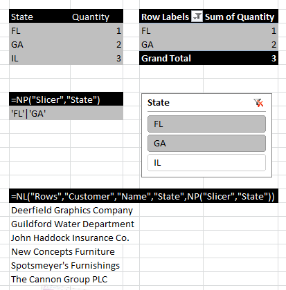
"Slicer"Returns an Excel Slicer in Arg1 that can be used as a filter in Jet functions when using a Cube data source.

EVAL

To increase performance, you can reduce cross-sheet references. The following NP evaluates the formula in cell of D5 from a worksheet called Options. =NP("Eval","=Options!$D$5")

This function is executed once on refreshing the report, rather than for every cell update. =NP("Eval","=Today()")

Performance can also be increased by not using volatile functions.
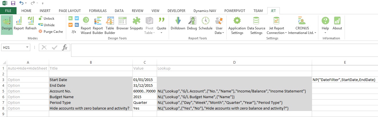
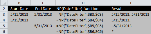
DATEFILTER

Results of using the NP(DateFilter) function, which can then be nested in other functions.
NP-1
INTEGERS

This NP(Integers) function will create rows with the numbers 1 through 10. =NL("Rows",NP("Integers",1,10))

JOIN

The following NP(Join) joins the strings from an array and creates the result "100|200|300|400" for potential use in another function. =NP("Join",{"100","200","300","400"},"|")

SPLIT

The following NP(Split) splits up the string "this|is|an|array" and creates the array {this, is, an, array}. =NP("Split", "this|is|an|array", "|")

COMPANIES

The following NP(Companies) function lists all the companies for the current data source in rows. =NL("Rows",NP("Companies"))
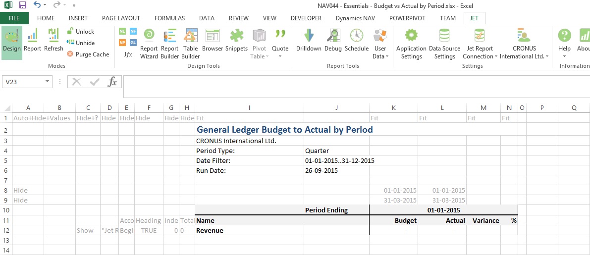
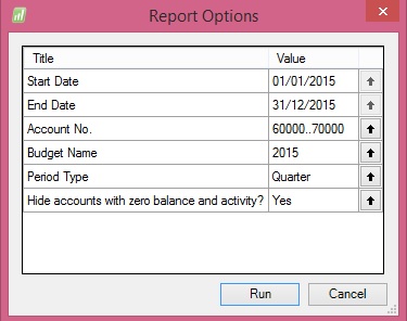
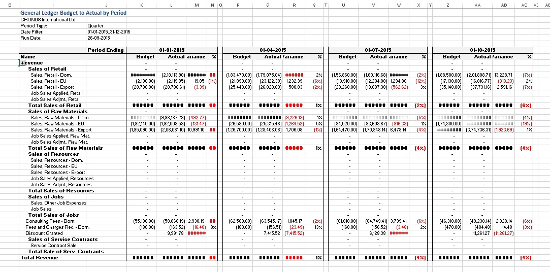
DATES

The use of NP(Dates) to create a set of column headers for a report. (Dates can also be placed in reverse order by putting the later date in first)
NP-2
DATASOURCES

This NP(DataSources) function will return a list of the data sources in use on the machine it is run on. =NL("Rows",NP("Datasources"))
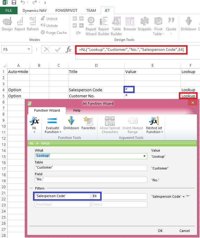
FORMULA

Used in conjunction with the NL(Table) function to define a calculated column in the table definition. For example: To determine available credit for a customer; if cell E6 contains the credit limit, and cell F6 contains the open credit, then =NP("Formula","=E6-F6") would be put in the field list of the NL(Table) definition

SLICER

The Slicer function works in conjunction with pivot tables and dashboards to provide information for filters when refreshing reports.
NP-3
Array Calculations

Arrays are lists of data values. You can obtain a string representing such a list from Jet using "Filter" as the What parameter in an NL function. The values in arrays returned by Jet are guaranteed to be unique. The resulting array might be a list of Customers or a list of Invoice Document numbers or any other list of data that match a set of filters. The array calculation operations of the NP function allow you to find different combinations of two arrays.

An example of when you would need an array calculation is listing the invoice document numbers where either the Type on an Invoice Line is "Item" for all item numbers, or the Type is "G/L Account" and the account number is 300. Both the Item numbers and the G/L Account numbers are stored in the same "No." field, so there is no single set of filters that will create this list of document numbers.

The array operations available in the NP function are "Difference", "Union" and "Intersect". The difference between two arrays consists of all of the elements that are in the first array but are not in the second. The union of two arrays consists of a single copy of all of the elements in both arrays with any duplicates eliminated. The intersection of two arrays is the set of elements that are common to both arrays. An example of the results of the array operations are listed in the table below.


Array 1 {100, 200, 300, 400, 500}Array 2 {400, 500, 900, 1000, 2000}
Difference{100, 200, 300}
Union{100, 200, 300, 400, 500, 900, 1000, 2000}
Intersect{400, 500}

=NL("Rows", NP("Union", NL("Filter","Customer","No.","Name","A*"), NL("Filter","Customer","No.","Name","B*")))

=NL("Rows","Customer","No.","Name","A*|B*")

The following formula creates a list down rows of the document numbers of all invoices where either the Type field is "Item", or it is "G/L Account" and the No. field is 2000.

=NL("Rows", NP("Union", NL("Filter","Sales Invoice Line","Document No.","Type","Item"), NL("Filter","Sales Invoice Line","Document No.","Type","G/L Account","No.","2000")))

You should be cautious using arrays because they are often not the easiest or fastest way to solve a problem. Example 1 is a good example of a query that does not require arrays, and will run much slower if you use them. Also remember that, with Jet Essentials 2015 and earlier, if NP("Union"), NP("Intersect"), or NP("Difference") are by themselves in a cell they will only return the first value from the array. You must put them inside NL("Rows") as in the examples above in order to correctly return all the data.

There are two more array operations that behave a bit differently than those listed above: "Split" and "Join". "Split" takes two text strings and splits the first string based on the second, resulting in an array. For instance, if you wanted to create a list of account numbers based on the string "1000+2000+3000", the formula would look like the following.

=NP("Split","1000+2000+3000","+")

The result would be the array {"1000","2000","3000"}. Note that this must be put inside an NL("Rows") as in the Union examples above in order to return all the data.

In the opposite scenario, if you have an array but would like to create a text string by joining each element of that array separated by a given string, you would use the "Join" operation. Using the same array, you can create a string for a filter with array values separated by the "|" character with the following formula.

=NP("Join",{"1000","2000","3000"},"|")

The result would be the text string "1000|2000|3000", which is a valid filter that you could pass into an NL function.

For Join and Split, Arg1 of the NP function is the value you want to manipulate and Arg2 is the character by which you want to join or split the value. If you experiment with these operations, you will find that you have an amazing amount of flexibility, especially when you use them in conjunction with the other array calculation formulas listed above.

Please note that the results of an NP("Join") may be very large and thus putting it directly inside another function may cause problems with Excels 256 character formula limit as in the following formula.

=NL("Rows",NP("Split",NP("Join",{"some","array","here"},"|"),"|"))

It is recommended that in a situation like this the NP("Join") be placed in a separate cell as in the following.

B2: =NP("Join",{"some","array","here"},"|")

B3: =NL("Rows",NP("Split",B2,"|"),"|"))

Stay tuned for usage of NP functions in Jet Reports.

I will come up with more details in my upcoming posts.

Friday 25 September 2015

Using NL( Lookup ) in Jet Reports Part-3

We have discussed regarding Lookup in my previous post. If you missed can find link here.

Using NL( Lookup ) in Jet Reports Part-1.

Using NL( Lookup ) in Jet Reports Part-2.

Continuing with more advanced usage I am here below.

Another useful feature of the NL(“Lookup”) function is the ability to specify how many records Jet Reports will go through in order to create a list of values.

By default, Jet Reports uses the value that is set for Maximum Lookup Records Scanned on the Jet Reports Options form. The default is 1,000 records. If the number of desired records to be searched is larger than this setting, the “ScanLimit=” keyword can be utilized.

To apply a scan limit, “ScanLimit=” must be placed in one of the FilterField parameters and then the desired number of records to be searched will be placed in the associated Filter parameter.

To create a Lookup function that will return all of the G/L Account Numbers in the first 5,000 records of a G/L transaction table, the function would look like this:
=NL(“Lookup”,”G/L Entry”,”G/L Account No.”,”ScanLimit=”,”5000”)

The NL("Lookup") function normally returns all values (for the particular field) that are present in the table specified.  For fields defined in NAV as "Option" fields, it may sometimes be desirable to display *all possible* value - regardless as to whether those values are present in the table or not.  For this, a useful feature is the "SmartLookup=" option (available in Jet Essentials 2012 R2 and later).

For example, the function:
=NL("Lookup","Item Ledger Entry","Entry Type")

Might provide a Lookup window that may not list all options depending upon data in the table.

By adding the "SmartLookup" option we could get a list of all options defined as option to that field.
 =NL("Lookup","Item Ledger Entry","Entry Type","SmartLookup=","TRUE")

Lookup-10

Stay tuned for more details in my upcoming posts

Using NL( Lookup ) in Jet Reports Part-2

We have discussed regarding Lookup in my previous post. If you missed can find link here.

Using NL( Lookup ) in Jet Reports Part-1.

I am continuing with more advanced usage here below.

In some instances it is also desirable to base the values that are displayed in one NL(“Lookup”) function on the results that were selected in another NL(“Lookup”) function.

An example of this could exist in a Sales Report. The viewer will have the ability to select a Salesperson Code to run the report for, and will also be able to specify Customer Numbers in order to filter the report further.

If only one Salesperson Code is selected, however, it may be undesirable to display Customer Numbers that are associated with other Salesperson Codes.

In this instance, two NL(“Lookup”) functions will be used, with the Customer Number filtered by the Salesperson Code so that the values are related. The first NL(“Lookup”) function, which will allow the selection of the Salesperson Code, will look like this:
Lookup-6

Lookup-7

The next NL(“Lookup”) function will give the viewer the ability to select from a list of Customer Numbers, but it will be filtered based on the Salesperson Code that was previously selected. This is done but inserting a normal filter into the function and referencing the cell containing the Salesperson Code that was previously selected by the viewer.

This addition would make the report look like this:
Lookup-8
After selecting Salesperson Code Filter when we open Customer List it will show lookup as below:
Lookup-9

Customer List is filtered out with Salesperson Code we selected using Salesperson List Lookup.

Will come up with more details in my upcoming post, stay tuned for more details.